How to Calculate Percentage in Excel

Microsoft Excel is a powerful ally for students, educators, and administrators managing complex grade sheets. While a manual calculator is fine for a single result, Excel allows you to automate thousands of calculations with a single formula, ensuring consistency and preventing human error.

The Foundations of Excel Percentages

Unlike a standard calculator where you multiply by 100 at the end, Excel treats percentages as a "formatting" layer over a decimal value. For example, the value 0.85 is mathematically identical to 85% in Excel's engine.

Method 1: The Classic Ratio

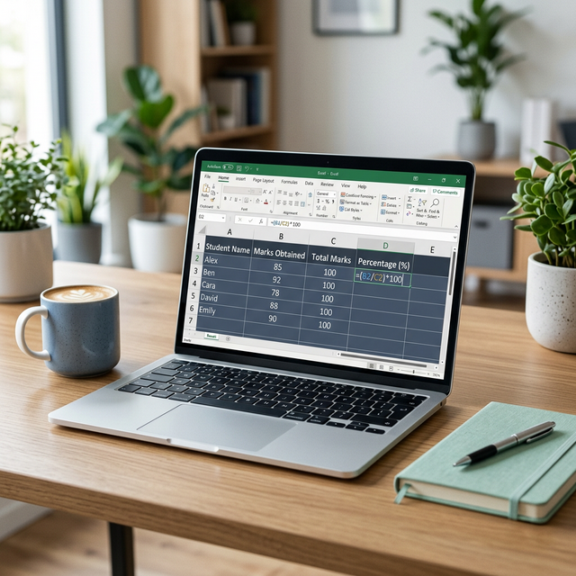
If your Obtained Marks are in cell A2 and the Maximum Possible Marks are in cell B2:

1. Click on cell C2.
2. Enter the formula: =A2/B2
3. Press Enter. You will likely see a decimal like 0.876.
4. Apply the Percentage Style: Click the % button in the 'Number' group on the Home tab (or press Ctrl+Shift+%).

Method 2: Handling Multiple Subjects

If you have marks for five subjects in cells A2 through E2 and a grand total possible of 500:

1. Formula: =SUM(A2:E2)/500
2. This automatically adds your scores and calculates the aggregate percentage against the total base.

Advanced Academic Excel Techniques

1. Conditional Formatting for "Pass/Fail"

You can make your spreadsheet "smart" by highlighting students who fall below a certain percentage.

• Select your percentage column.
• Go to Home > Conditional Formatting > Highlight Cell Rules > Less Than.
• Enter 40% (or your pass mark) and select "Red Fill". Now, any failing grade will be instantly flagged visually.

2. Calculating Percentage Change (Improvement)

If you want to track how much a student improved from Mid-terms (B2) to Finals (C2):

• Formula: =(C2-B2)/B2
• A positive result shows growth, while a negative result shows a decline in performance.

3. Handling Errors with IFERROR

If a cell is empty or has a zero in the total marks column, Excel will show a #DIV/0! error. To keep your sheet clean, use:

• =IFERROR(A2/B2, "-")
• This tells Excel to show a simple dash instead of an ugly error message if the data is missing.

Pro Tips for Efficiency

• The Flash Fill shortcut: Once you enter a formula in the first row, double-click the small green square (the "fill handle") at the bottom-right of cell C2. Excel will instantly populate the formula for every student in your list.
• Absolute References: If your Total Marks is in a single cell (like $F$1), use a dollar sign in your formula (e.g., =A2/$F$1) to lock that reference when dragging the formula down.

---

Frequently Asked Questions